TL;DR: This post summarizes how modern linear attention architectures (e.g., Mamba, RWKV, RetNet) can be unified under the Test-Time Training (TTT) framework. It reviews how TTT leverages Fast Weight Programming to update hidden states on-the-fly via gradient descent (exemplified by the Delta Rule), and contrasts this dynamic memory approach with traditional RNNs and the computationally expensive Self-Attention mechanism.
1. Test Time Training (TTT)
1.1 Formulation of the Test Time Training
Test-Time Training (TTT) retrieves data relevant to the input from the training set or knowledge base during inference to fine-tune the model, improving its performance in dynamic scenarios.
Consider a one-dimensional sequence of $N$ tokens $\mathbf{x} = [x_1, x_2, \dots, x_N]$, where each token $x_i \in \mathbb{R}^d$. Following attention formulation, each input token $x_i$ is projected into query ($q_i$), key ($k_i$), and value ($v_i$) vectors. For clarity, we assume all these vectors $q_i, k_i, v_i \in \mathbb{R}^d$.
TTT introduces a neural network with rapidly adaptable weights (fast weights) that are updated during both training and inference to dynamically store context information. This contrasts with the slow weights (i.e., model parameters) that are frozen during inference. Formally, TTT defines fast weights in the form of a neural network: $f_W (\cdot) : \mathbb{R}^d \to \mathbb{R}^d$ parameterized by the fast weights $W$, and it involves two primary operations:
Update operation: $$ W \leftarrow W - \eta\nabla_W \mathcal{L} $$ where $\mathcal{L}(\cdot, \cdot)$ is a loss function between the transformed key $f_W (k)$ and the value $v$, commonly Mean Squared Error, designed to encourage the network to associate keys with corresponding values (KV-Binding). $\eta$ is the learning rate. Intuitively, this learning objective is to encode the KV cache into a neural memory with fixed state size as accurate as possible.
Output rule: $$ o = f_W (q) $$ where the updated fast weights $W$ are used to compute the output vector $o$ given the query $q$. The per-token TTT layer iteratively performs the update and apply operations on each token $x_i$ in sequence.
1.2 Example: The DeltaRule under TTT framework
DeltaNet reinterprets the recurrence as online gradient descent on a reconstruction objective:
$$ \mathcal{L}_t(\mathbf{S}) = \frac{1}{2}|\mathbf{S}^\top\boldsymbol{k}_t - \boldsymbol{v}_t|^2 $$
Taking a gradient step with learning rate $\beta_t$ gives:
$$ \begin{aligned} \mathbf{S}_t &= \mathbf{S}_{t-1} - \beta_t \nabla_\mathbf{S}\mathcal{L}_t(\mathbf{S}_{t-1}) \\ &= \mathbf{S}_{t-1} - \beta_t \boldsymbol{k}_t (\mathbf{S}_{t-1}^\top \boldsymbol{k}_t - \boldsymbol{v}_t)^\top \\ &= \mathbf{S}_{t-1} - \beta_t \boldsymbol{k}_t \boldsymbol{k}_t^\top \mathbf{S}_{t-1} + \beta_t \boldsymbol{k}_t \boldsymbol{v}_t^\top \\ &= (\mathbf{I}-\beta_t\boldsymbol{k}_t\boldsymbol{k}_t^\top) \mathbf{S}_{t-1} + \beta_t\boldsymbol{k}_t\boldsymbol{v}_t^\top \end{aligned} $$
This rule—the classical delta rule—treats $\mathbf{S}$ as a learnable associative memory that continually corrects itself toward the mapping $\boldsymbol{k}_t \mapsto \boldsymbol{v}_t$.
2. Attention mechanisms under TTT framework
2.1 Unified Linear Attention mechanisms under TTT framework
An overview of different attention mechanisms through the lens of state updating rules and their learning objective under the TTT framework. All normalizer terms and activation/kernel functions are ignored for brevity.
| Model | Objective $\mathcal{L}$ | Update rule $\mathbf{S}_t = \mathbf{S}_{t-1} - \nabla_{\mathbf{S}_{t-1}}\mathcal{L}$ |
|---|---|---|
| LA | $-\langle\mathbf{S}_{t-1}^\top \boldsymbol{k}_t, \boldsymbol{v}_t\rangle$ | $\mathbf{S}_t = \mathbf{S}_{t-1}+\boldsymbol{k}_t\boldsymbol{v}_t^\top$ |
| RetNet | $-{\beta_t}\langle\mathbf{S}_{t-1}^\top \boldsymbol{k}_t, \boldsymbol{v}_t\rangle+\frac{1}{2}|\sqrt{1-\mathbf{\alpha}}~\mathbf{S}_{t-1}|_F^2$ | $\mathbf{S}_t = \alpha\mathbf{S}_{t-1}+{\beta_t}\boldsymbol{k}_t\boldsymbol{v}_t^\top$ |
| Mamba2 | $-{\beta_t}\langle\mathbf{S}_{t-1}^\top \boldsymbol{k}_t, \boldsymbol{v}_t\rangle+\frac{1}{2}|\sqrt{1-\mathbf{\alpha}_t}\mathbf{S}_{t-1}|_F^2$ | $\mathbf{S}_t = \alpha_t\mathbf{S}_{t-1}+{\beta_t}\boldsymbol{k}_t\boldsymbol{v}_t^\top$ |
| GLA | $-\langle\mathbf{S}_{t-1}^\top \boldsymbol{k}_t, \boldsymbol{v}_t\rangle+\frac{1}{2}|\sqrt{\operatorname{Diag}(\boldsymbol{1}-\boldsymbol{\alpha}_t)}\mathbf{S}_{t-1}|_F^2$ | $\mathbf{S}_t = \operatorname{Diag}(\boldsymbol{\alpha}_t)\mathbf{S}_{t-1}+\boldsymbol{k}_t\boldsymbol{v}_t^\top$ |
| HGRN2 | $-\langle\mathbf{S}_{t-1}^\top (\mathbf{1-\boldsymbol{\alpha}}_t), \boldsymbol{v}_t\rangle+\frac{1}{2}|\sqrt{\operatorname{Diag}(\boldsymbol{1}-\boldsymbol{\alpha}_t)}\mathbf{S}_{t-1}|_F^2$ | $\mathbf{S}_t = \operatorname{Diag}(\boldsymbol{\alpha}_t)\mathbf{S}_{t-1}+(\mathbf{\boldsymbol{1}-\boldsymbol{\alpha}}_t)\boldsymbol{v}_t^\top$ |
| Longhorn | $\frac{1}{2}|\mathbf{S}_{t-1}^\top \boldsymbol{k}_t-\boldsymbol{v}_t |^2_{\operatorname{Diag}(\boldsymbol{\beta}_t)}$ | $\mathbf{S}_t = (\mathbf{I} -\frac{\boldsymbol{\beta}_t}{\boldsymbol{1}+\boldsymbol{\beta}_t\boldsymbol{k}_t^\top\boldsymbol{k}_t}\boldsymbol{k}_t\boldsymbol{k}_t^\top)\mathbf{S}_{t-1}+{\beta_t}\boldsymbol{k}_t\boldsymbol{v}_t^\top$ |
| Comba | $\frac{{\beta_t}}{2}|\mathbf{S}_{t-1}^\top \boldsymbol{k}_t -\boldsymbol{v}_t|^2+\frac{1}{2}|\sqrt{1-\mathbf{\alpha}_t}\mathbf{S}_{t-1}|_F^2$ | $\mathbf{S}_t = (\alpha_t -\beta_t\boldsymbol{k}_t\hat{\boldsymbol{k}}_t^\top)\mathbf{S}_{t-1}+{\beta_t}\boldsymbol{k}_t\boldsymbol{v}_t^\top$ |
| RWKV7 | $\frac{1}{2}|\mathbf{S}_{t-1} ^\top\tilde{\boldsymbol{k}}_t-\boldsymbol{v}_t|^2+\frac{1}{2}|\sqrt{\operatorname{Diag}(\boldsymbol{1}-\boldsymbol{\alpha}_t)}\mathbf{S}_{t-1}|_F^2$ | $\mathbf{S}_t = (\operatorname{Diag}(\boldsymbol{\alpha}_t)-(\boldsymbol{b}_s\odot\hat{\boldsymbol{k}}_s)\hat{\boldsymbol{k}}_t^\top)\mathbf{S}_{t-1}+{\boldsymbol{k}}_t\boldsymbol{v}_t^\top$ |
| GDN | $\frac{{\beta_t}}{2}|\tilde{\mathbf{S}}_{t-1}^\top \boldsymbol{k}_t-\boldsymbol{v}_t|^2$ | $\mathbf{S}_t = (\mathbf{I}-{\beta}_t\boldsymbol{k}_t\boldsymbol{k}_t^\top)\alpha_t\mathbf{S}_{t-1}+{\beta}_t\boldsymbol{k}_t\boldsymbol{v}_t^\top$ |
| KDA | $\frac{\beta_t}{2}|\tilde{\mathbf{S}}_{t-1}^\top {\boldsymbol{k}_t}-\boldsymbol{v}_t|^2$ | $\mathbf{S}_t = (\mathbf{I} -\beta_t\boldsymbol{k}_t\boldsymbol{k}_t^\top)\operatorname{Diag}(\boldsymbol{\alpha}_t)\mathbf{S}_{t-1}+{\beta_t}\boldsymbol{k}_t\boldsymbol{v}_t^\top$ |
For GDN and KDA, the update can be viewed as performing a Stochastic Gradient Descent (SGD) process on the decayed state
$\tilde{\mathbf{S}}$, that is,$\mathbf{S}_t = \tilde{\mathbf{S}}_{t-1} - \nabla_{\tilde{\mathbf{S}}_{t-1}}\mathcal{L}$, where$\tilde{\mathbf{S}}_{t-1}$is decayed by scalar or fine-grained gate.
2.2 Sequence Modeling Paradigms under TTT framework
Here is a comparison of three sequence modeling approaches from the perspective of Test-Time Training:
| Initial state | Update rule | Output rule | Cost | |
|---|---|---|---|---|
| Naive RNN | $s_0 = \text{vector}()$ | $s_t = \sigma (\theta_{ss}s_{t-1} + \theta_{sx}x_t)$ | $z_t = \theta_{zs}s_t + \theta_{zx}x_t$ | $O(1)$ |
| Self-attention | $s_0 = \text{list}()$ | $s_t = s_{t-1}.\text{append}(k_t, v_t)$ | $z_t = V_t\text{softmax}(K_t^T q_t)$ | $O(t)$ |
| Naive TTT | $W_0 = f.\text{params}()$ | $W_t = W_{t-1} - \eta\nabla \ell(W_{t-1}; x_t)$ | $z_t = f(x_t; W_t)$ | $O(1)$ |
Self-attention differs fundamentally from RNNs and TTT in how it manages memory. While RNNs and TTT compress historical context into a fixed-size hidden state (resulting in constant $O(1)$ cost per token), Self-attention maintains an ever-growing list known as the Key-Value (KV) cache. Its “update rule” is trivial—simply appending new keys and values—but its “output rule” requires scanning the entire history to compute the attention matrix. This lack of compression grants Self-attention superior expressivity for long contexts, but it comes at the price of linear computational complexity $O(t)$ per token as the sequence lengthens.
3. TTT and Fast Weight Programming
3.1 What is Fast Weight Programming?
Below is the abstract from the paper ‘Using Fast Weights to Attend to the Recent Past’:
Until recently, research on artificial neural networks was largely restricted to systems with only two types of variable: Neural activities that represents the current or recent input and weights that learn to capture regularities among input, outputs and payoffs. However, synapses have dynamics at many different time-scales. Artificial neural networks might benefit from variables that change slower than activities but much faster than the standard weights. These “fast weights” can be used to store temporary memories of the recent past and they provide a neurally plausible way of implementing the type of attention to the past. By using fast weights we can avoid the need to store copies of neural activity patterns.
 Fast Weight Programming is a mechanism that dynamically adjusts neural network weights based on the input sequence, enabling the model to maintain a form of short-term memory.
Fast weights separates RNN’s memory into two components to free up the its hidden state for computation rather than memorization:
Fast Weight Programming is a mechanism that dynamically adjusts neural network weights based on the input sequence, enabling the model to maintain a form of short-term memory.
Fast weights separates RNN’s memory into two components to free up the its hidden state for computation rather than memorization:
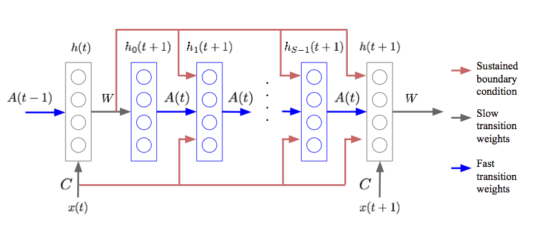
- Slow weights ($W$): Standard RNN weights, learned via backpropagation, holding long-term knowledge.
- Fast weights ($A(t)$): Dynamic weights changing at every timestep via a Hebbian-like rule, holding short-term memory of the recent past.
Update Rule (Hebbian Learning): The fast weights $A(t)$ are updated based on the outer product of the hidden state: $$ A(t+1) = \lambda A(t) + \eta h(t)h(t)^T $$ where $\lambda$ is the decay rate and $\eta$ is the learning rate.
3.2 Connection between TTT and Fast Weight Programming
TTT can be viewed as a generalized framework for Fast Weight Programming. In TTT, the “hidden state” effectively serves as the fast weights that are updated on-the-fly. While the original Fast Weights used a specific Hebbian update rule, TTT employs gradient descent on a local objective (like the reconstruction loss in DeltaNet) to update these weights. This perspective unifies various linear attention models: they are essentially maintaining a fast-changing memory matrix (the KV cache or state $S$) optimized to represent the recent context, distinct from the static model parameters (slow weights).
reference
- Ba, J. et al. (2016) “Using Fast Weights to Attend to the Recent Past.” arXiv. Available at: https://doi.org/10.48550/arXiv.1610.06258.
- Sun, Y. et al. (2025) “Learning to (Learn at Test Time): RNNs with Expressive Hidden States.” arXiv. Available at: https://doi.org/10.48550/arXiv.2407.04620.
- Zhang, T. et al. (2025) “Test-Time Training Done Right.” arXiv. Available at: https://doi.org/10.48550/arXiv.2505.23884.
- Hu, J. et al. (2025) “Test-Time Learning for Large Language Models.” arXiv. Available at: https://doi.org/10.48550/arXiv.2505.20633.
- Team, K. et al. (2025) “Kimi Linear: An Expressive, Efficient Attention Architecture.” arXiv. Available at: https://doi.org/10.48550/arXiv.2510.26692.